Probabilistic Roadmaps
Introduction
The probabilistic roadmap method is a fairly simple sampling based path planning method, compared to the other sampling based algorithms, RRT and RRT*. It was introduced in the paper titled Probabilistic Roadmaps for Path Planning in High-Dimensional Configuration Spaces, and the invention of the PRM method is credited to Lydia E. Kavraki.
As this is a sampling based algorithm, it involves randomly sampling points in a given space.
This algorithm is divided into two phases, namely, the learning phase and the query phase.
-
In the learning phase, the roadmap containing nodes and edges is generated. These nodes and edges are entirely inside the search space and do not overlap with obstacles.
-
In the query phase, graph based algorithms, like A* and Dijkstra’s algorithms, are used on the probabilistic roadmap to find the optimal path.
It is important to first get an intuition of the algorithm before moving on to the pseudocode.
How it works
Learning Phase
The robot in question can only take certain configurations and positions in a given space. The set of all these configurations is called the configuration space or C-space.
In a given space, the first step is to randomly generate a point. It is then checked whether this point is in C-space or not.
If it is in C-space, we add this point to the graph by connecting it to all the points in the graph that are within a specific radius from the generated point by a straight line. It also checks whether this line is in free space, and only forms this connection if it is.

Source: Mathematical Problems in Engineering
In the above diagram, a node \(q_i\) was randomly generated. Nodes within the radius \(r_{\eta}\) are searched for and connected to \(q_i\) through edges.
This process is then repeated as many times as necessary. As the number of samples tends to infinity, the likelihood that the graph is a true road map tends to 100%.
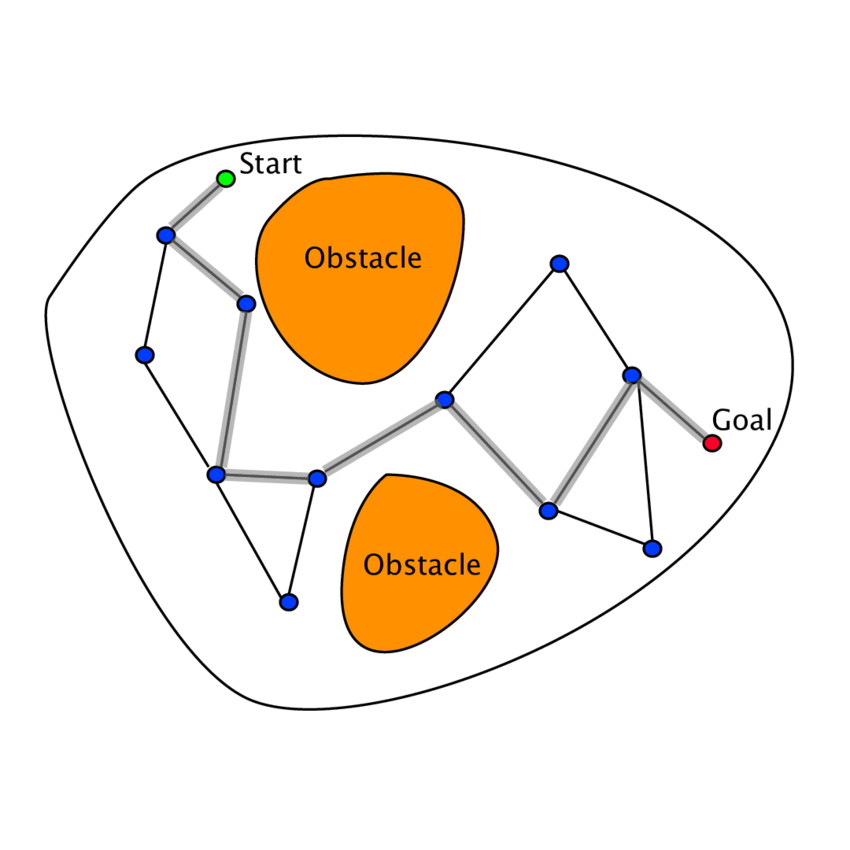
Once this is done, we add the start node and the goal node by joining a line from each of the two to the closest node in the graph to each of them.
Query Phase
This phase involves using the nodes of the roadmap generated in the learning phase as points on a graph and use graph based algorithms like A* and Dijkstra to come up with an optimal path for the robot to take.
Given the start and goal configurations, \(s\) and \(g\), the method tries to connect them to two nodes \(\tilde{s}\) and \(\tilde{g}\) in the graph. If succesful, the method tries to find the optimal path from \(s\) to \(g\) using graph based algorithms.
We have already covered graph based algorithms separately so you can refer to those for how they work.
One interesting thing to note is that the learning phase and query phase can be interwoven, i.e., the two phases don’t need to be carried out sequentially.
For example, we might first create a small roadmap and then apply graph based algorithms on it. We might simultaneously perform the learning phase and connect new nodes generated to the path to create a more optimal path as both phases are being carried out simultaneously.
For this section, however, we will assume the learning phase has been carried out before performing query phase.
Let’s now look at the pseudocode that describes the algorithm. The functions used in the pseudocode are explained in our page on the RRT* algorithm, under the section “Functions used in Pseudocode”.
Pseudocode
The following pseudocode only performs the learning phase for the PRM algorithm. The query phase has not been included in the pseudocode.
def PRM(n, r, x_init, x_goal):
    V = []
    E = []
    for i in range(n):
        x_rand = SampleFree()
        U = Near(V, E, x_rand, r)
        V.append(x_rand)
        U.Sort(distance(x_rand))
        for u in U:
            if [[x_rand, u], [u, x_rand]] not in E:
                if CollisionFree(x_rand, u):
                    E.append([[x_rand, u], [u, x_rand]])

    return V, E
In this psuedocode, the function U.Sort(distance(x_rand)) sorts the list U according to the Euclidean distance between each element of the list and x_rand, in increasing order.