Optimal Rapidly Exploring Random Trees (RRT*)
In the year 2011, Sertac Karaman and Emilio Frazzoli in their paper Sampling-based Algorithms for Optimal Motion Planning, introduced three new path planning algorithms that improved upon the existing algorithms. These were, namely, optimal rapidly exploring random trees (RRT*), optimal probabilistic road mapping (PRM*), and rapidly exploring random graphs (RRG).
The most popular algorithm among these is the RRT* algorithm, that is heavily based on the RRT algorithm, and has some improvisions, and provides a more optimal solution.
Let’s now look at the RRT* algorithm that was originally proposed in the paper along with the pseudo code. All the mathematical notations and functions in the paper are clearly explained here.
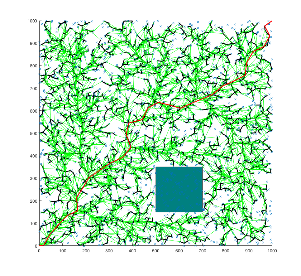
The following image shows the RRT* algorithm applied on a 2D graph.
 Courtesy: SAI VEMPRALA
Intuition
The node sampling and selection process is exactly the same as RRT, wherein a point is randomly generated and a node is created at that point or at a specified maximum distance from the existing node, whichever is closer.
However, the difference is where the connection is made. We assign every node a cost function that denotes the length of the shortest path from the start node. We then search for nodes inside a circle of given radius r centred at the newly sampled point.
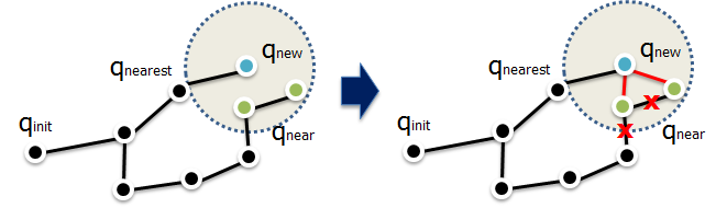
We then rearrange the connections such that they minimize the cost function and optimize the path. This can rearrange the graph in such a way that we get the shortest path.
 Courtesy: Joon’s lectures
In the image above, after rearranging the connections, the path to the green points, i.e., \(q_{near}\) is shorter through the red connections than through the earlier connections.
Pseudocode
The following is the pseudocode for the RRT* algorithm. An explanation of all the unique functions used in the pseudocode is explained below.
def RRT_Star(V, E, r, c):
    V = [x_init]
    E = []
    # G = (V, E)
    for i in range(1, n):
        x_rand = SampleFree()
        x_nearest = Nearest(V, E, x_rand)
        x_new = Steer(x_nearest, x_rand)
        if ObstacleFree(x_nearest, x_new):
            X_near = Near(V, E, x_new, r)
            # list of all nodes at radius r
            V.append(x_new)
            x_min = x_nearest
            c_min = cost(x_nearest) + c(Line(x_nearest, x_new))
            # the cost of the nearest node to new node
            # to check whether to change paths

            for x_near in X_near:
                if CollisionFree(x_near, x_new)*Cost(x_near)+c(Line(x_near, x_new)) < c_min:
                    x_min = x_near
                    c_min = Cost(x_near) + c(Line(x_near, x_new))
                    # update c_min, because we now need to find nodes that are closer than this new x_new

            E.append([x_min, x_new])

            for x_near in X_near:
                if CollisionFree(x_new, x_near)*Cost(x_new) + c(Line(x_new, x_near)) < Cost(x_near):
                    x_parent = Parent(x_near)
                    E.remove([x_parent, x_near])
                    E.append([x_new, x_near])
                    # remove all edges between nodes (in radius r) and their parents and join them with x_new
                    # this is the step of reconnection of edges
    return V, E
Functions used in Pseudocode
SampleFree()
The function SampleFree() is used to return a randomly sampled node. The samples are generally assumed to be drawn from a uniform distribution.
Suppose the set of sample space is given as \(\Omega\) and for each \(\omega \in \Omega\),
is a map from \(\Omega\) to a sequence of points \(\mathcal{X_{free}}\), which is the obstacle-free space.
Nearest()
This function is used to return the nearest node in the graph.
Let’s say that our tree is a graph \(G=(V,E)\) where \(V\) and \(E\) are sets of vertices and edges of our tree, where \(V\subset \mathcal{X}\). We take a point \(x\in \mathcal{X}\) such that the function \(Nearest:(G,x)\mapsto v \in V\) returns the node \(v\) in \(V\) that is closest to the point \(x\) in terms of a distance function, such as Euclidean distance, i.e.,
where \(argmin_{v \in V} ||x-v||\) means that the value \(v\) in \(V\) is returned such that the distance \(||x-v||\) is minimum.
Near()
This function is used to find the nodes in the graph in a fixed radius in order to rearrange the connections such that we get the optimal path.
Let’s say the radius is \(r\) such that \(r\in \mathbb{R}\). The function \(Near:(G,x,r)\mapsto V'\subseteq V\) returns the vertices \(V'\) in \(V\) that are contained in a circle of radius \(r\) centred \(x\), i.e.,
where \(\mathfrak{B}_{x,r}\) is the set of all points within the fixed radius \(r\) centred at \(x\).
Steer()
This function is the one that creates a new node that is at a maximal distance from the nearest node in the direction of the sampled node (or it’s equal to the sampled node itself, if it’s closer than this distance).
Suppose we have two points \(x,y\in \mathcal{X}\). The function \(Steer:(x,y)\mapsto z\) returns a point \(z \in \mathcal{X}\) such that \(z\) is closer to \(y\) than \(x\) is. This will be such that \(z\) minimizes the distance \(||z-y||\) and at the same time maintains the distance \(||z-x||\leq\eta\) for the predefined maximal distance \(\eta > 0\), i.e.,
Line()
The Line() function is used to denote a straight line, i.e., given two points \(x_1,x_2\in \mathbb{R}^d\),
Parent()
The Parent() function is used to denote the parent node of a given node in a tree, i.e., given a tree \(G=(V,E)\), \(Parent:V\mapsto V\) is a function that maps a vertex \(v\in V\) to the unique vertex \(u\in V\) such that \((u,v)\in E\).
Note that if \(v_0 \in V\) is the start node of \(G\), then, by convention, \(Parent(v_0)=v_0\).
Cost()
This is function that makes RRT* different from RRT. As mentioned before, we assign each node a cost that is a function of the distance along the path from the start node. It’s given as follows.If \(Cost:V\mapsto \mathbb{R}^+\) is a function that maps the vertex \(v_0\mapsto V\) to the cost of the unique path from the root of the tree to \(v\), then
where \(c\) is a function that transforms the length value of the \(Line\) into a cost
Note that if \(v_0\) is the start node or root vertex of \(G\), then, by convention, \(Cost(v_0)=0\).
CollisionFree()
CollisionFree(x,x') returns True if the line segment joining x and x’ lies in \(\mathcal{X_{free}}\), where \(x,x'\in \mathcal{X}\) and False otherwise.
Visual comparison between RRT and RRT*
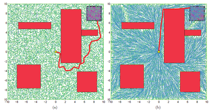
The following image shows the RRT and RRT* algorithms applied on a 2D graph with obstacles. The plot on the left is RRT and the plot on the right is RRT*. As one can see, the RRT* algorithm provides a more optimal solution to the path planning problem.
 Courtesy: András Gyimesi
A flowchart summary of the RRT* algorithm
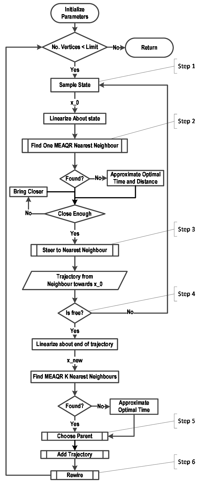
The following flowchart provides a visual summary of the optimal rapidly exploring random trees algorithm.
 Courtesy: Nir Rikovitch